|
|
|
|
|
|
|
|
|
|
|
|
|
|
|
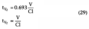
Zero-order processes and first-order processes are the basis of
mathematical pharmacokinetic models. Processes such as the flow of a river or a
person's consumption of oxygen happen at a constant rate. These are called zero-order
processes. The rate of change (dx/dt) for a zero-order process is defined
by the following equation:
Equation 17 states that the rate of change is constant. If x represents an amount
of drug and t represents time, the units of k are amount per time. To find the value
of x at time t, x(t), we can compute it as the integral of the equation from time
0 to time t:
x(t) = x0
+ kt (18)
In Equation 18, x0
is the value of x at time 0. This is the equation
of a straight line with a slope of k and an intercept of x0
.
Many processes occur at a rate proportional to the amount. For
example, the interest payment on a loan is proportional to the outstanding balance,
and the rate at which water drains from a bathtub is proportional to the amount of
water in the tub. These are examples of first-order processes.
The rate of change in a first-order process is only slightly more complex than for
a zero-order process:
The units of k are 1/time, because x on the right side already includes the units
for the amount. The value of x at time t, x(t) can be computed as the integral from
time 0 to time t:
x(t) = x0
ekt
(20)
In Equation 20, x0
is the value of x at time 0. If k is greater than
0, x(t) increases exponentially. If k is less than 0, x(t) decreases exponentially.
In pharmacokinetics, k is negative because concentrations decrease over time. For
clarity, the minus sign is usually explicit, and k is expressed as a positive number.
The identical equation for pharmacokinetics, with the minus sign explicitly written,
is:
x(t) = x0
e−kt
(21)
Figure 3-12
shows the relationship
between x and time as described by Equation 21. In Figure
3-12
, x continuously decreases over time, but the slope of the curve continuously
increases (i.e., becomes less negative). Taking the natural logarithm of both sides
of Equation 21 gives the following:
This is the equation of a straight line, as shown in Figure
3-13
, for which the vertical axis is ln(x(t)), the horizontal axis is t,
the intercept is ln(x0
), and the slope of the line is -k.
How long does it take for x to go from some value, x1 , to one half of that value, x1 /2. Because k is the slope of a
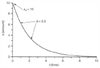 Figure 3-12
Exponential decay curve, as given by x(t) =
x0
e−kt
, plotted on standard axes, with x0
= 10 and k = 0.5.
Figure 3-12
Exponential decay curve, as given by x(t) =
x0
e−kt
, plotted on standard axes, with x0
= 10 and k = 0.5.
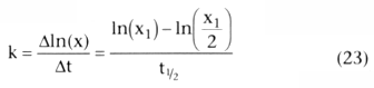
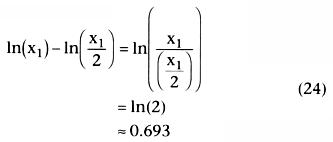
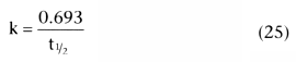
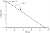 Figure 3-13
The same exponential decay curve, x(t) =
x0
e−kt
, as in Figure
3-12
is plotted on a log y axis.
Figure 3-13
The same exponential decay curve, x(t) =
x0
e−kt
, as in Figure
3-12
is plotted on a log y axis.
It is possible to analyze volumes and clearances for each organ in the body and to construct models of pharmacokinetics by assembling the organ models into physiologically and anatomically accurate models of the entire animal. These models typically assume blood flows throughout the system as zero-order processes and drug transfers between the blood and tissues as first-order processes. Figure 3-14 shows such a model for thiopental in rats.[6] Subsequent studies have shown that individual tissue volumes and blood flows can be scaled up from rats to humans, resulting in accurate models of human pharmacokinetics. [7] This illustrates the potential utility of physiologically based pharmacokinetic models in developing human pharmacokinetic models from animal models.
Models that work with individual tissues are mathematically cumbersome and do not offer a better prediction of plasma drug concentration than models that lump the tissues into a few compartments. If the goal is to determine how to give drugs to obtain therapeutic plasma drug concentrations, all that is needed is to mathematically relate dose to plasma concentration. For this purpose, conventional compartmental models are usually adequate.
Compartmental models are built on the same basic concepts as physiologic models, but with gross simplifications. The one-compartment model see in Figure 3-15 contains a single volume and a single clearance, as though humans were built like buckets. For anesthetic drugs, we resemble several buckets connected by pipes. These situations are usually modeled using two- or three-compartment models (see Fig. 3-15 ). The volume to the right in the two-compartment model and in the center of the three-compartment model is the central volume. The other volumes are the peripheral volumes, and the sum of all the volumes is the volume of distribution at steady state. The clearance leaving the central compartment for the outside is the central or metabolic clearance. The clearances between the central compartment and the peripheral compartments are the intercompartmental clearances.
Think of the body as a bucket into which we pour drug. The amount of drug poured into the bucket is x0 (x at time 0). The initial concentration is x0 /V, and V is the volume of fluid in the bucket. Returning to Equation 1, if we know the concentration we want to achieve, the target concentration, CT , and the volume in the bucket, V, we can calculate the dose to achieve CT by rearranging the definition of concentration: Dose = CT × V. This topic is discussed further in Chapter 12 .
We can assume that the fluid is being pumped out of the bucket at a constant rate, which we call clearance, Cl. What is the rate, dx/dt, at which drug is flowing out of
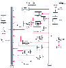 Figure 3-14
Physiologic model for thiopental in rats. The pharmacokinetics
of distribution into each organ has been individually determined. The components
of the model are linked by zero-order (flow) and first-order (diffusion) processes.
(From Ebling WF, Wada DR, Stanski DR: From piecewise to full physiologic
pharmacokinetic modeling: Applied to thiopental disposition in the rat. J Pharmacokinet
Biopharm 22:259–292, 1994.)
Figure 3-14
Physiologic model for thiopental in rats. The pharmacokinetics
of distribution into each organ has been individually determined. The components
of the model are linked by zero-order (flow) and first-order (diffusion) processes.
(From Ebling WF, Wada DR, Stanski DR: From piecewise to full physiologic
pharmacokinetic modeling: Applied to thiopental disposition in the rat. J Pharmacokinet
Biopharm 22:259–292, 1994.)

 Figure 3-15
One-, two-, and three-compartment mammillary models.
Figure 3-15
One-, two-, and three-compartment mammillary models.


Because this is a first-order process, 
,
and the integral of this gives the amount of drug at time t in terms of the amount
at time 0: x(t) = x0
e−kt
.
If we divide both sides by V and remember that x/V is the definition
of concentration, we get the equation that relates concentration after an intravenous
bolus to time and initial concentration:
C(t) = C0
e−kt
(30)
This equation defines the concentration over time curve
for a one-compartment model, and it has the log-linear shape seen in Figure
3-13
. We can calculate the clearance, Cl, in one of two ways. First,
we can calculate V by rearranging the definition of concentration: V =
dose/initial concentration = dose/C0
. Referring to
Equation 28, if we measure the slope, -k, we can calculate clearance as k
× V. A more
 Figure 3-16
A one-compartment model is similar to that in Figure
3-3
but has an increased volume of distribution. After drug administration,
concentrations fall more slowly in this model than in the model shown in Figure
3-3
.
Figure 3-16
A one-compartment model is similar to that in Figure
3-3
but has an increased volume of distribution. After drug administration,
concentrations fall more slowly in this model than in the model shown in Figure
3-3
.
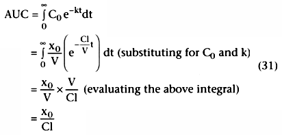
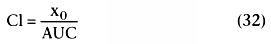
 Figure 3-17
A one-compartment model is similar to that in Figure
3-3
but has increased clearance. After drug administration, concentrations
fall faster in this model than in the model shown in Figure
3-3
.
Figure 3-17
A one-compartment model is similar to that in Figure
3-3
but has increased clearance. After drug administration, concentrations
fall faster in this model than in the model shown in Figure
3-3
.
When an infusion is given at an input rate of I, the plasma concentration
rises as long as the rate of drug going into the body, I, exceeds the rate at which
drug leaves the body, C × Cl, in which C is the drug concentration.
When I = C × Cl, drug is going in and coming out
at the same rate, and drug concentration in the body is at steady state. We can
calculate the concentration at steady state by observing that the rate of drug going
in must equal the rate of drug coming out. From Equation 6, we know that the rate
of drug metabolism at steady state is as follows:
Metabolic rate = C∞
Cl (33)
In Equation 33, C∞
is the arterial concentration at steady state.
By definition, the infusion rate at steady state must equal the metabolic rate,
and the infusion rate, I, at steady state therefore must be I =
C∞
Cl. Solving this for the concentration at steady
state, C∞
gives I/Cl. The steady-state concentration during an
infusion is the rate of drug input divided by the clearance. It follows that to
calculate the infusion rate that can achieve a given target concentration, CT
,
at steady state, the infusion rate must be CT
× Cl.
This topic is discussed further in Chapter
12
.

is similar in
form to the equation describing the concentration after a bolus injection: 
.
Volume is a scalar relating bolus to initial concentration, and
During an infusion, the rate of change in the amount of drug,
x, is the rate of inflow, I, minus the rate of outflow, k × x.
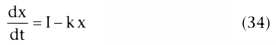
We can calculate x at any time t as the integral from time 0 to time t. Assuming
that x0
= 0 (i.e., starting with no drug in the body), the result is this:
As t → ∞, e-kt
→ 0, and Equation 35 reduces to the following:
How long does it take to reach 50% of the final steady-state concentration (i.e.,
to reach a concentration of 
) during an infusion? From
Equation 36, we know that 
. Substituting

for x(t) in Equation 35, we obtain the following:
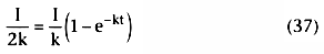
Solving Equation 37 for t, we get 
. Equation 26 showed
that the half-life, t½
, after a bolus injection was
.
Here, we have a parallel between boluses and infusions. During an infusion, it
takes one half-life to reach 50% of the steady-state concentration. Similarly, it
takes two half-lives to reach 75%, three half-lives to reach 88%, and five half-lives
to reach 97% of the steady-state concentration. By four or five half-lives, the
patient is typically considered to be at steady state, although the concentrations
only asymptotically approach the steady-state value.
In intravenous drug delivery, all of the drug reaches the systemic circulation. When drugs are given by a different route, such as orally, transdermally, epidurally, or intramuscularly, the drug must first reach the systemic circulation. Oral drugs may be metabolized by first-pass hepatic metabolism before reaching the systemic circulation. Transdermally applied drugs may be sloughed off with the stratum corneum without being absorbed. We cannot assume that the dose given to the patient is the same as the dose that reaches the systemic circulation when working with alternative routes of drug delivery. The dose that reaches the systemic circulation is the administered dose times f, the fraction that is bioavailable.
Alternative routes of drug delivery are often modeled by assuming
the drug is absorbed from a reservoir or depot, usually modeled as an additional
compartment with a monoexponential rate of transfer to the systemic circulation:
A(t) = fDoral
ka
e−ka
t
(38)
In Equation 38, A(t) is the absorption rate at time t, f is the fraction bioavailable,
Doral
is the dose taken orally (or intramuscularly or applied to the skin),
and ka
is the absorption rate constant. Because the integral of ka
e−ka
t
is 1, the total amount of drug absorbed
is f × Doral
. To compute the concentrations
over time, we first reduce the problem to differential equations (e.g., Equations
19 and 34) and then integrate. The differential equation for the amount, x, with
oral absorption into a one-compartment disposition model follows:
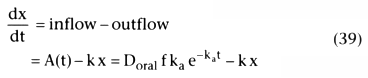
This is the rate of absorption at time t, A(t), minus the rate of exit, k x. To
solve for the amount of drug, x, in the compartment at time t, we integrate this
from 0 to time t, knowing that x(0) = 0:
Equation 40 describes the amount of drug in the systemic circulation when absorbed
from some depot, such as the stomach, an intramuscular injection, or the skin, or
from an epidural dose. To describe the concentrations, rather than amounts of drug,
it is necessary to divide both sides of Equation 40 by V, the volume of distribution.
This discussion covers the standard pharmacokinetic equations for one-compartment models. The one-compartment model introduces the concepts of rate constants and half-lives and relates them to the physiologic concepts of volume and clearance. Unfortunately, none of the drugs used in anesthesia can be accurately characterized by one-compartment models. Distribution of anesthetic drugs into and out of peripheral tissues plays a crucial role in the time course of anesthetic drug effect. To describe intravenous anesthetics, we must extend the one-compartment model to account for distribution into tissues.
The plasma concentrations over time after an intravenous bolus resemble the curve in Figure 3-18 . In contrast to Figure 3-13 , Figure 3-18 is not a straight line even though it is plotted on a log y axis. This curve has the characteristics common to most drugs when given by intravenous bolus. First, the concentrations continuously decrease over time. Second, the rate of decline is initially steep but continuously becomes less steep, until we get to a portion that has a log-linear form.
For many drugs, three distinct phases can be distinguished. There is a rapid-distribution phase (see Fig. 3-18, solid line ) that begins immediately after the bolus injection.
 Figure 3-18
Concentration versus time relationship shows a very rapid
initial decline after bolus injection. The terminal log-linear portion is seen only
after most of the drug has left the plasma. This is characteristic of most anesthetic
drugs. Different line types highlight the rapid, intermediate, and slow (log-linear)
portions of the curve.
Figure 3-18
Concentration versus time relationship shows a very rapid
initial decline after bolus injection. The terminal log-linear portion is seen only
after most of the drug has left the plasma. This is characteristic of most anesthetic
drugs. Different line types highlight the rapid, intermediate, and slow (log-linear)
portions of the curve.
The presence of three distinct phases after bolus injection is a defining characteristic of a mammillary model with three compartments. It is possible to develop hydraulic models, as shown in Figure 3-19 , for intravenous drugs.[8] In this model, there are three tanks, corresponding (see Fig 3-19, left to right ) with the slowly equilibrating peripheral compartment, the central compartment (i.e., the plasma, into which drug is injected), and the rapidly equilibrating peripheral compartment. The horizontal pipes represent intercompartmental clearance or (for the pipe draining onto the page) metabolic clearance. The volumes of each tank correspond with the volumes of the compartments for fentanyl. The cross-sectional areas of the pipes correlate with fentanyl's systemic and intercompartmental clearances. The height of water in each tank corresponds to drug concentration.
Using this hydraulic model, we can follow the processes that decrease drug concentration over time after bolus injection. Initially, drug flows from the central compartment
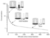 Figure 3-19
Hydraulic model of fentanyl pharmacokinetics. Drug is
administered into the central tank, from which it can distribute into two peripheral
tanks, or it may be eliminated. The volume of the tanks is proportional to the volumes
of distribution. The cross-sectional area of the pipes is proportional to the clearance.
(Adapted from Youngs EJ, Shafer SL: Basic pharmacokinetic and pharmacodynamic
principles. In White PF [ed]: Textbook of Intravenous
Anesthesia. Baltimore, Williams & Wilkins, 1997, p 10.)
Figure 3-19
Hydraulic model of fentanyl pharmacokinetics. Drug is
administered into the central tank, from which it can distribute into two peripheral
tanks, or it may be eliminated. The volume of the tanks is proportional to the volumes
of distribution. The cross-sectional area of the pipes is proportional to the clearance.
(Adapted from Youngs EJ, Shafer SL: Basic pharmacokinetic and pharmacodynamic
principles. In White PF [ed]: Textbook of Intravenous
Anesthesia. Baltimore, Williams & Wilkins, 1997, p 10.)
After the concentration in the central compartment decreases below those of the rapidly and slowly equilibrating compartments (see Fig. 3-19, dotted line ), the only method of decreasing the plasma concentration is metabolic clearance. The return of drug from both peripheral compartments to the central compartment greatly slows the rate of decrease in plasma drug concentration.
Curves that continuously decrease over time with a continuously
increasing slope (i.e., curves such as those in Fig.
3-18
and Fig. 3-19
)
can be described by a sum of exponentials. In pharmacokinetics, one way of denoting
this sum of exponentials is to say that the plasma concentration over time is as
follows:
C(t) = Ae−αt
+ Be−βt
+ Ce−γt
(41)
The main reason that polyexponential equations are used is that they describe the plasma concentrations observed after bolus injection, except for the misspecification in the first minute. Compartmental pharmacokinetics is strictly empirical; the models describe the data, not the processes by which the observations came to be. Fortunately, polyexponential equations permit us to use many of the one-compartment ideas previously developed, with some generalization of the concepts. This involves translating Equation 41 into a model of volumes and clearances that has an appealing, if not necessarily accurate, physiologic flavor.
Equation 41 says that the concentrations over time are the algebraic
sum of three separate functions: Ae-αt
, Be-βt
,
and Ce-γt
. Typically, α > β > γ by about
one order of magnitude. We can graph each of these functions separately and their
sum, as shown in Figure 3-20
.
At time 0 (t = 0), Equation 41 reduces to the following:
C0
= A + B + C (42)
The sum of the coefficients A, B, and C equals the concentration immediately after
a bolus.
Special significance is often ascribed to the smallest exponent. This exponent determines the slope of the final log-linear portion of the curve. When the medical literature refers to the half-life of a drug, unless otherwise stated, the half-life is the terminal half-life (i.e., 0.693/smallest exponent). However, the terminal half-life for drugs with
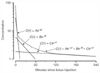 Figure 3-20
The disposition of a three-compartment model (i.e., triexponential
model) consists of the sum of three monoexponential functions. The concentrations
over time are the algebraic sum of three separate functions, Ae-αt
,
Be-βt
, and Ce-γt
. Typically, α > β
> γ by about one order of magnitude. The functions can be graphed separately
(solid lines) and as their sum (dotted
line).
Figure 3-20
The disposition of a three-compartment model (i.e., triexponential
model) consists of the sum of three monoexponential functions. The concentrations
over time are the algebraic sum of three separate functions, Ae-αt
,
Be-βt
, and Ce-γt
. Typically, α > β
> γ by about one order of magnitude. The functions can be graphed separately
(solid lines) and as their sum (dotted
line).
Constructing pharmacokinetic models represents trade-offs in accurately describing the data, having confidence in the results, and mathematical tractability. Adding exponents to the model usually provides a better description of the observed concentrations. However, adding more exponent terms usually decreases our confidence in how well we know each coefficient and exponential and greatly increases the mathematical burden of the models. This is why most pharmacokinetic models are limited to two or three exponents.
Part of the continuing popularity of polyexponential models of
pharmacokinetics is that they can be mathematically transformed from the admittedly
unintuitive exponential form in equation to a more easily intuited compartmental
form (see Fig. 3-15
). Micro
rate constants, expressed as kij
, define the rate of drug transfer from
compartment i to compartment j. Compartment 0 is a compartment outside the model,
and k10
is the micro rate constant for processes acting through metabolism
or elimination that irreversibly remove drug from the central compartment (i.e.,
analogous to k for a one-compartment model). The intercompartmental micro rate constants
(e.g., k12
, k21
) describe the movement of drug between the
central and peripheral compartments. Each compartment has at least two micro rate
constants, one for drug entry and one for drug exit. The micro rate constants for
the two- and three-compartment models can be seen in Figure
3-15
. The differential equations describing the rate of change for the
amount of drugs in compartments 1, 2, and 3 follow directly from the micro rate constants.
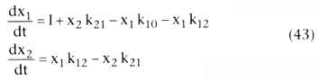
For the two-compartment model, the differential equations for each compartment are
as follows:
For the three-compartment model, the differential equations for each compartment
are as follows:
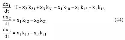
In Equation 44, I is the rate of drug input. An easy way to model pharmacokinetics
is to convert the previous differential equations to difference equations, so that
dx becomes Δx and dt becomes Δt. With a Δt of 1 second, the error
from linearizing the differential equations is less than 1%. In this way, desktop
computers can easily simulate pharmacokinetics using a spreadsheet.
For the one-compartment model, k was both the rate constant and the exponent. For multicompartment models, the relationships are more complex. Interconversion between the micro rate constants and the exponents becomes exceedingly complex as more exponents are added, because every exponent is a function of every micro rate constant and vice versa. These interconversions can be found in the Excel spreadsheet ("convert.xls"), which can be downloaded from http://anesthesia.stanford.edu/pkpd.
The plasma is not the site of drug effect for anesthetic drugs. There is a time lag between drug concentration in plasma and that in the effect site. For example, one significant difference between fentanyl and alfentanil is the more rapid onset of alfentanil's drug effect. The black bar in the upper graph of Figure 3-21 shows the duration of a fentanyl infusion.[9] Rapid arterial samples document the rise in fentanyl concentration. The time course of electroencephalographic (EEG) effect lags 2 to 3 minutes behind the rapid rise in arterial concentration. This lag is called hysteresis. The plasma concentration peaks at the moment the infusion is turned off. After the peak plasma concentration (see Fig. 3-21 ), the fentanyl concentration rapidly decreases. However, the offset of fentanyl drug effect again lags well behind the decrease in concentration. The lower graph in Figure 3-21 shows the same study design in a patient receiving alfentanil. Because of alfentanil's rapid blood-brain equilibration, there is less hysteresis with alfentanil than with fentanyl.
Typically, the relationship between the plasma and the site of
drug effect is modeled with an effect-site model, as shown in Figure
3-22
. The site of drug effect is connected to the plasma by a first-order
process. The following equation relates effect site concentration to plasma concentration:
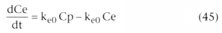
In Equation 45, Ce is the effect site concentration, Cp is the plasma drug concentration,
and ke0
is the rate constant for elimination of drug from the effect site.
It is most easily understood in terms of its reciprocal, 0.693/ke0
, the
half-time for equilibration between the plasma and the site of drug effect.
The constant ke0 has a large influence on the rate of rise of drug effect, the rate of offset of drug effect, and the dose that is required to produce the desired drug effect. The mathematical basis of these relationships is explored in Chapter 12 .
|
|
|
|
|
|
|
|
|
|
|
|
|